2.2 Hierarchical Data and the Closure Property
As we have seen, pairs provide a primitive “glue” that we can use to
construct compounf data objects. The figure below shows a standard way
to visualize a pair – in this case, the pair formed by (cons 1 2).
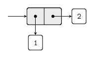
Tikz code here
In this representation, which is called box-pointer notation, each
object is shown as a pointer to a box. The box for a primitive
object contains a representation of the object. The box for a pair is
actually a double box, the left part containing (a pointer to) the
car of the pair and the right part containing the cdr.
We have already seen that cons can be used to combine not only
numbers but pairs as well. As a consequence, pairs provide a universal
building block from which we can construct all sorts of data
structures. The figures below show two ways to use pairs to combine
the numbers 1, 2, 3, and 4.
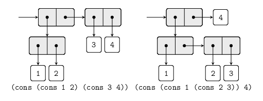
Tikz code here
The ability to create pairs whose elements are pairs is the essence of
list structure;s importance as a representational tool. We refer to
this as the closure property of cons. In general, an operation
for combining data objects satisfies the closure property if the
result of combining things with that operation can themselves be
combined using the same operation. Closure is the key to power in any
means of combination becuase it permits us to create hierarchical
structures – structures made up of parts, which themselves are made
up of parts, and so on.
2.2.1 Representing Sequences
A sequence is an ordered collection of data objects. A
straightforward representation of sequences using pairs is illustrated
below, where the sequence 1, 2, 3, 4 is represented as a chain of
pairs. The car of each pair is the corresponding item in the chain,
and the cdr of the pair is the next pair in the chain. The cdr of
the final pair signals the end of the sequence by pointing to a
distinguished value that is not a pair, represented in box-and-pointer
diagrams as a diagonal line and in programs as the value of the
variable nil (or rather '() in mit-scheme). The entire sequence is
constructed by nested cons operations:
(define nil '())

(cons 1
      (cons 2
            (cons 3
                  (cons 4 nil))))
Tikz code here
Such a sequence of pairs, formed by nested conses, is called a
list, and Scheme provides a primitive list to help construct
lists. [In this book, we use list to mean a chain of pairs
terminated bu the end-of-list marker. In contrast, the term list
structure refers to any data structure made out of pairs, not just to
lists.]
In general,
(list <a1> <a2> ... <an>)is equivalent to
(cons <a1>
      (cons <a2>
            (cons ...
                  (cons <an> '()) ...)))
Lisp systems conventionally prints lists by printing the sequence of
elements, encolsed in parentheses, for example (1 2 3 4).
We can think of car as selecting the first item in the list, and of
cdr as selecting the sublist consisting of all but the first item.
Nested applications of car and cdr can be used to etract the
second, third, and subsequent items in the list. The constructor cons
makes a list like the original one, but with an additional item at the
beginning.
List operations
The use of pairs to represent sequences of elements as list is
accompanied by conventional programming techniques for manipulating
lists bu successively “cdring down” the list. For example, the
procedure list-ref takes as arguments a list and a number n and
returns the nth item of the list. It is customary to number the
elements of the list beginning with 0. The method for computing
list-ref is the following: For n = 0, list-ref should return the
car of the list. Otherwise, list-ref should return the (n-1)th
item of the cdrlist.
(define (list-ref items n)
    (if (= n 0)
        (car items)
        (list-ref (cdr items) (- n 1))))
Often we cdr down the whole list. To aid in this, Scheme includes a
primitive predicate null?, which tests whether its arguments is the
empty list. The procedure length, which returns the number of items
in a list, illustrates this typical pattern of use:
(define (length items)
    (if (null? items)
        0
        (+ 1 (length (cdr items)))))
Another conventional programming technique is to “cons up” an answer
list while cdring down a list, as in the procedure append, which
takes two lists as arguments and combines their elements to make a new
list:
(define (append list1 list2)
    (if (null? list1)
        list2
        (cons (car list1)
              (append (cdr list1) list2))))
Mapping over lists
One extremely useful operation is to apply some transformation tp each element in a list and generate the list of results. For instance, the following procedure scales each number in a list by a given factor:
(define (scale-list items factor)
    (if (null? items)
        '()
        (cons (* (car items) factor)
              (scale-list (cdr items factor)))))
We can abstract this general idea and capture it as a common pattern
expressed as a high-order procedure. The higher-order procedure here
is called map. It take as arguments a procedure of one argument and
a list, and returns a list of the results produced by applying the
procedure to each element in the list:
(define (map proc items)
    (if (null? items)
        '()
        (cons (proc (car items))
              (map proc (cdr items)))))
Now we can give a new definition of scale-list in terms of map:
(define (scale-list items factor)
    (map (lambda (x) (* x factor))
         items))
Scheme standardly provides a map procedure that is more general: it
takes as arguments a procedure of n arguments together with n
lists and applies the procedure with all the first elements of the
lists as arguments, then all the second elements, and so on, returning
a list of the results. For example:
(map + (list 1 2 3) (list 40 50 60) (list 700 800 900))
; (741 852 963)
The procedure map is an important construct, not only because it
captures a common pattern, but because it establishes a higher-level
of abstraction in dealing with lists. In the original definition of
scale-list, the recursive structure of the program draws attention
to the element-by-element processing of the list. Defining scale-list
in terms of map suppresses that level of detail and emphasizes that
scaling transforms a list of elements to a list of results. The
difference between the two definitions is not that the computer is
performing a different process (it isn’t) but that we think about the
process differently.
2.2.2 Hierarchical structures
The represenation of sequences in terms of lists generalizes naturally
to represent sequences whose elements may themselves be sequences. For
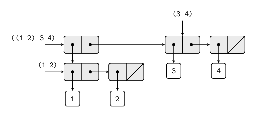
example, we can regard the object ((1 2) 3 4) constructed by
(cons (list 1 2 ) (list 3 4))as a list of three items, the first if which is itself a list, (1 2).
Indeed, this is suggested by the form in which the result is printed
by the interpreter. The following figure shows the representation of
this structure in terms of pairs.
Tikz code here
Another way to think of sequences whose elements are sequences is as trees. The elements of the sequences are the branches of the tree, and elements that are themselves sequences are subtrees. The following figure shows the structure viewed as a tree.
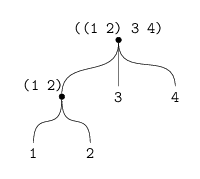
Tikz code here
Recursion is a natural tool for dealing with tree strucutres, since we
can often reduce operations on trees to operations on their branches,
which reduce in turn to operations on the branches of the branches,
and so on, until we reach the leaves of the trees. As an example,
compare the length procedure above with the count-leaves procedure,
which returns the total number of leaves of a tree:
(define x (cons (list 1 2) (list 3 4)))

(length x)
; 3

(count-leaves x)
; 4

(length (list x x))
;2

(count-leaves (list x x))
; 8
The implement count-leaves, recall the recursive plan for computing
length:
lengthof the empty list is 0lengthof a listxis 1 pluslengthof thecdrofx
The count-leave procedure is similar:
count-leavesof the empty list is 0count-leavesof a treexiscount-leavesof thecarofxpluscount-leavesof thecdrofxcount-leavesof a leaf is 1
To aid in writing recursive procedues on trees, Scheme provides the
primitive predicate pair?, which tests whether its argument is a
pair. So presenting the count-leaves procedure:
(define (count-leaves x)
    (cond ((null? x) 0)
          ((not (pair? x)) 1)
          (else (+ (count-leaves (car x))
                   (count-leaves (cdr x))))))
Mapping over trees
Just as map is a powerful abstraction for dealing with sequences,
map together with recusion is a powerful abstraction for dealing
with trees. For instance the scale-tree procedure, analogous to
scale-list above, takes as arguments a numeric factor and a tree
whose leaves are numbers. It returns a tree of the same shape, where
each number is multiplied by the factor. The recursive plan for
scale-tree is similar to the one for count-leaves
(define (scale-tree tree factor)
    (cond ((null? tree) '())
          ((not (pair? tree)) (* tree factor))
          (else (cons (scale-tree (car tree) factor)
                      (scale-tree (cdr tree) factor)))))

(scale-tree (list 1 (list 2 (list 3 4) 5) (list 6 7))
            10)
; (10 (20 (30 40) 50) (60 70)
Another way to implement scale-tree is to regard the tree as a
sequence of sub-trees in turn, and use map. We map over the sequence,
scaling each sub-tree in turn, and return the list of results. In the
base case, where the tree is a leaf, we simple multiply by the factor:
(define (scale-tree tree fator)
    (map (lambda (sub-tree)
             (if (pair? sub-tree)
                 (scale-tree sub-tree factor)
                 (* sub-tree factor)))
          tree))
Many tree operations can be implemented by similar combinations of sequence operations and recursion.
2.2.3 Sequences as Conventional Interfaces
In this section we introduce another powerful design principle for working with data structures – the use of conventional interfaces.
In Section 1.3
we saw how program abstractions, implemented as higher-order
procedures, can capture common patterns in programs that deal with
numerical data. Our ability to formulate analogous operations for
working with compound data dependeds crucially on the style in which
we manipulate our data structures. Consider, for example, the
following procedure, analogous to the count-leaves procedure,
which takes a tree as argument and computes the sum of the square of
the leaves that are odd:
(define (sum-odd-squares tree)
    (cond ((null? tree) 0)
          ((not (pair? tree))
           (if (odd? tree) (square tree) 0))
          (else (+ (sum-odd-squares (car tree))
On the surface, this procedure is very different from the following one, which constructs a list of all the even Fibonacci numbers $\mathrm{Fib}(k)$, where $k$ is less than or equal to a given integer $n$:
(define (even-fibs n)
    (define (next k)
        (if (> k n)
            '()
            (let ((f (fib k)))
                 (if (even? f)
                     (cons f (next (+ k 1)))
                     (next (+ k 1))))))
    (next 0))
Despite the fact that these two procedures are structurally very different, a more abstract description of the two computations reveals a great deal of similarity. The first program
- emumerates the leaves of a tree;
- filters them, selecting the odd ones;
- squares each of the selected ones; and
- accumulates the results using
+, starting with 0.
The second program
- enumerates the integers from 0 to $n$;
- computes the Fibonacci number for each integer;
- filters them, selecteding the even ones; and
- accumulates the results using
cons, starting with the empty list.
A signal-processing engineer would find it natural to conceptualize these processes in terms of signals flowing through a cascade of stages, each of which implements part of the program plan, as shown below.

Tikz code here
In sum-odd-squares, we begin with an enumerator which creates a
“signal” consisting of the leaves of a given tree. This signal is
passed through a filter which eliminates all but the odd elements.
The resulting signal is in turn passed through a map, which is a
“transducer” that applies the square procedure to each element. The
output of the map is then feed to an accumulator, which combines
the elements using +, starting from an initial 0. The plan for
even-fibs is analogous.
Unfortunately, the two procedure definitions above fail to exhibit
this signal-flow structure. For instance, if we examine the
sum-odd-squares procedure, we find that the enumeration is
implemented partly by the null? and the pair? test and partly by
the tree recursive structure of the procedure. Similarly, the
accumulation is found partly in the tests and partly in the addition
used in the recursion. In general, there are no distinct parts of
either procedure that corresponds to the elements in the signal-flow
description. Our two procedures decompose the computations in a
different way, spreading the enumeration over the program and mingling
it with the map, the filter and the accumulation. If we could
orgranise our program to make the signal-flow strucutre manifest in
the procedures we write, this would increase the conceptual clarity of
the resulting code.
Sequence Operations
The key to organizing programs so as to more clearly reflect the
signal-flow strucutre is to concentrate on the “signals” that flow
from one stage in the process to the next. If we represent these
signals as lists, then we can use list operations to implement the
processing at each of the stages. For instance, we can implement the
mapping stages of the signal-flow diagrams using the map procedure
(map square (list 1 2 3 4 5))
; (1 4 9 16 25)
Filtering a sequence to select only those elements that satisfy a given predicate is accomplished by
(define (filter predicate sequence)
    (cond ((null? sequence) '())
          ((predicate (car sequence))
           (cons (car sequence)
                 (filter predicate (cdr sequence))))
          (else (filter predicate (cdr sequence)))))

(filter odd? (list 1 2 3 4 5))
; (1 3 5)
Accumulation can be implemented by
(define (accumulate op initial sequence)
     (if (null? sequence)
         initial
         (op (car sequence)
             (accumulate op initial (cdr sequence)))))

(accumulate + 0 (list 1 2 3 4 5))
; 15

(accumulate * 1 (list 1 2 3 4 5))
; 120

(accumulate cons '() (list 1 2 3 4 5))
; (1 2 3 4 5)
All that remains ti implement signal-flow diagrams is to enumerate
the sequence of elements to be processed. For even-fibs we need to
generate the sequence of integers in a given range, which we can do
as follows:
(define (enumerate-interval low high)
    (if (> low high)
        '()
        (cons low (enumerate-interval (+ low 1) high))))

(enumerate-interval 2 7)
; (2 3 4 5 6 7)
To enumerate the leaves of a tree, we can use
(define (enumerate-tree tree)
    (cond ((null? tree) '())
          ((not (pair? tree)) (list tree))
          (else (append (enumerate-tree (car tree))
                        (enumerate-tree (cdr tree))))))

(enumerate-tree (list 1 (list 2 (list 3 4)) 5))
; (1 2 3 4 5)
Now we can refomulate sum-odd-squares and even-fibs as in the
signal-flow diagrams.
(define (sum-odd-squares tree)
    (accumulate +
                0
                (map square
                     (filter odd?
                             (enumerate-tree tree)))))

(define (even-fibs n)
    (accumulate cons
                '()
                (filter even?
                        (map fib
                             (enumerate-interval 0 n)))))
The value of expressing programs as sequences opeartions is that this helps us make program designs that are modular, that is, designs that are constructed by combining relatively independent pieces. We can encourage modular design by providing a library of standard components together with a conventional interface for connection the components in flexible ways.
Sequences, implemented here as lists, serve as a conventional interface that permits us to combine processing modules. Additionally, when we uniformly represent strucutres as sequences, we have localized the data ststructure dependencies in our program to a small number of sequence operations. By changing these we can experiment with alternative representations of sequences, while leaving the overall design of our programs intact. We will exploit this capability in Section 3.5 when we generalize the sequence-processing paradigm to admit infinite sequences.
Nested Mappings
We can exten the sequence paradigm to include many computations that are commonly expressed using nested loops. Consider this problem: given a positive integer $n$, find all ordered pairs of distinct positive integers $i$ and $j$, where $1\le j\lt i\le n$, such that $i+j$ is prime.
A natural way to organize this computation is to generate the sequence of ordered pairs of positive integers less than or equal to $n$, filter to select those pairs whose sum is prime, and then, for each pair $(i,j)$ that passes throught the filter, produce the triple $(i,j,i+j)$.
Here is a way to generate the sequence of pairs: for each integer
$i\le n$, enumerate the integers $j\lt i$, and for each such $i$ and
$j$ generate the pairs $(i, j)$. In terms of sequence operations we
map along the sequence (enumerate-interval 1 n). For each $i$ in
this sequence, we map along the sequence
(enumerate-interval 1 (- i 1)). For each $j$ in this latter sequence,
we generate the pair (list i j). This gives us a sequence of pairs
for ach $i$. Combining all the sequences for all the $i$ (by
accumulating with append) procedures the required sequence of pairs:
(accumulate append
            `()
            (map (lambda (i)
                   (map (lambda (j) (list i j))
                        (enumerate-interval 1 (- i 1))))
                 (enumerate-interval 1 n)))
The combination of mapping and accumulating with append is so
common in this sort of program that we will isolate it as a separate
procedure:
(define (flatmap proc seq)
   (accumulate append `() (map proc seq)))
Now filter this sequence of pairs to find those whose sum is prime. The filter predicate is called for each element of the sequence; its argument is a pair and it must extract the integers from the pair. Thus, the predicate to apply to each element in the sequence is
(define (prime-sum? pair)
   (prime? (+ (car pair) (cadr pair))))
Finally, generate the sequence of results by mapping over the filtered pairs using the following procedure, which constructs a triple consisting of the two elements of the pair along with their sum:
(define (make-pair-sum pair)
    (list (car pair) (cadr pair) (+ (car pair) (cadr pair))))
Combining all these steps:
(define (prime-sum-pairs n)
    (map make-pair-sum
         (filter prime-sum?
                 (flatmap
                  (lambda (i)
                      (map (lambda (j) (list i j))
                           (enumerate-interval 1 (- i 1))))
                  (enumerate-interval 1 n)))))
Nested mappings are also useful for sequences other than those that enumerate intervals. Suppose we wish to generate all the permutations of a set $S$. For instance, the permutations of $\{1,2,3\}$ are $\{1,2,3\}$, $\{1,3,2\}$, $\{2,1,3\}$, $\{2,3,1\}$, $\{3,1,2\}$ and $\{3,2,1\}$. Here is a plan for generating the permutations of $S$: for each item $x$ in $S$, recursively generate the sequence of permutations of $S-x$, and adjoin $x$ to the font of each one. This yields, for each $x$ in $S$, the seqeuence of permutations of $S$ that begins with $x$. Combining these sequences for all $x$ gives all permuations of $S$:
(define (permutations s)
    (if (null? s)
        (list `())
        (flatmap (lambda (x)
                   (map (lambda (p) (cons x p))
                        (permutations (remove x s))))
                 s)))
Notice how this strategy reduces the problem if generation
permutations of $S$ to the problem of generating the permutations of
sets with fewer elements then $S$. In the terminal case, we work our
way down to the empty list, which represents a set of no elements. For
this, we generate (list '()), which is a sequence with one item,
namely the set with no elements. The remove procedure used in
permutations return all the items in a given sequence except for a
given item. This can be expressed as a simple filter:
(define (remove item sequence)
    (filter (lambda (x) (not (= x item)))
            sequence))
2.2.4 Example: A Picture Language
This section presents a simple language for drawing pictures that
illustrates the power of data abstraction and closure, and also
exploits higher-order procedures in an essentia way. In this language,
the data objected being combined are represented as procedures rather
than as list structure. Just as cons, which statisfies the closure
property, allowed us to easily build arbitrarily complicated list
structure, the operations in this language, which also satisfy the
closure property, allow us to easily build arbitrarily complicated
patterns.
The picture language
In the picture language there is only one kind of element, called a
painter. A painter draws an image that is shifted and scaled to fit
within a designated parallelogram-shaped frame. For example there’s a
primitive painter we’ll call wave that makes a crude line drawing,
as show below.
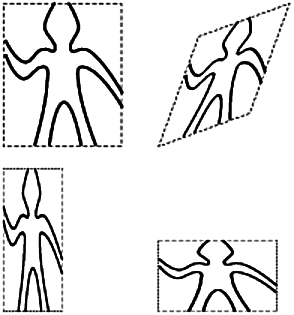
The actual shape of the drawing depends on the frame – all four
images above are produced by the same wave painter, but with respect
to four different frames.
To combine images, we use various operations that construct new
painters from given painter. For example, the beside operation takes
two painters and produces a new, compound painter that draws the first
painter’s image in the left half of the frame and the second painter’s
image in the right half of the frame.
Similarly below takes two painters and produces a compound painter
that draws the first painter’s image below the second painter’s image.
Some operations transform a single painter to produce a new painter.
For example, flip-vert takes a painter and produces a painter that
draws its image upside-down, and flip-horiz produces a painter that
draws the original painter’s image left-to-right reversed.
The figure below shows the drawing of a painter called wave4 that is
built up in two stages starting from wave:
(define wave2 (beside wave (flip-vert wave)))
(define wave4 (below wave2 wave2))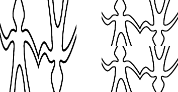
Scheme/Script-fu code here
In building up a complex image in this manner we are exploiting the
fact that painters are closed under the language’s means of
combination. The beside or below of two painters is itself a
painter; therefore, we can use it as an element in making more complex
painters. As with building up list structure using cons, the closure
of our data under the means of combination is crucial to the ability
to create complex structures while using only a few operations.
Once we can combine painters, we would like to be able to abstract
typical patterns of combining painters. We will implement the painter
operations as Scheme procedures. This means that we don’t need a
special abstraction mechanism in the picture language: Since the means
of combination are ordinary Scheme procedures, we automatically have
the capability to do anything with painter operations that we can do
with procedures. For example, we can abstract the pattern in wave4
as
(define (flipped-pairs painter)
  (let ((painter2 (beside painter (flip-vert painter))))
       (below painter2 painter2)))
and define wave4 as an instance of this pattern:
(define wave4 (flipped-pairs wave))We can aslo define recursive operations. Here’s one that makes painters split and branch towards the right as shown in the figures below:
(define (right-split painter n)
  (if (= n 0)
      painter
      (let ((smaller (right-split painter (- n 1))))
        (beside painter (below smaller smaller)))))
We can also produce balanced patterns by branching upwards as well as towards the right, also show in the figures below:
(define (corner-split painter n)
  (if (= n 0)
      painter
      (let ((up (up-split painter (- n 1)))
            (right (right-split painter (- n 1))))
        (let ((top-left (beside up up))
              (bottom-right (below right right))
              (corner (corner-split painter (- n 1))))
             (beside (below painter top-left)
                     (below bottom-right corner))))))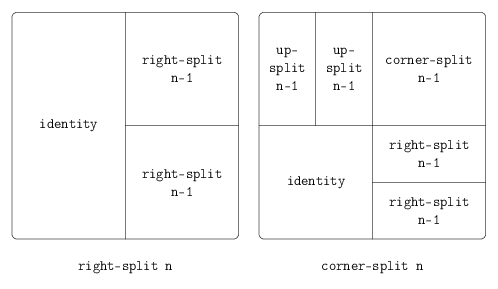
Tikz code here
right-split:
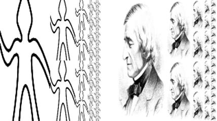
corner-split:
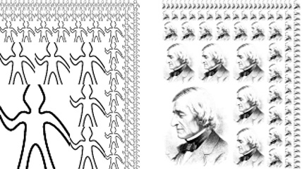
Scheme/Script-fu code here
By placing four copies of a corner-split appropriately, we obtain a
pattern called square-limit, whose application to wave and
rogers as show below:
(define (square-limit painter n)
  (let ((quarter (corner-split painter n)))
    (let ((half (beside (flip-horiz quarter) quarter)))
      (below (flip-vert half) half))))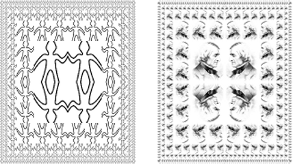
Scheme/Script-fu code here
Higher-order operations
In addition to abstracting patterns of combining painters, we can work at a higher level, abstracting patterns of combining painter operations. That is, we can view the painter operations as elements to manipulate and can write means of combination for these elements – procedures that take painter operations as arguments and create new painter operations.
For example, flipped-pairs and square-limit each arrange four copies
of a painter’s image in a square pattern; they differ only in how they
orient the copies. One way to abstract this pattern of painter
combination is with the following procedure, which takes four
one-argument painter operations and produces a painter operation that
transforms a given painter with those four operations and arranges the
results in a square. tl, tr, bl, and br are the
transformations to apply to the top left copy, the top right copy, the
bottom left copy, and the bottom right copy, respectively.
(define (square-of-four tl tr bl br)
  (lambda (painter)
    (let ((top (beside (tl painter) (tr painter)))
          (bottom (beside (bl painter) (br painter))))
      (below bottom top))))
Then flipped-pairs can be defined in terms of square-of-four as
follows:
(define (flipped-pairs painter)
  (let ((combine4 (square-of-four identity flip-vert
                                  identity flip-vert)))
    (combine4 painter)))
or equivalently
(define flipped-pairs
  (square-of-four identity flip-vert identity flip-vert))
and square-limit can be expressed as
(define (square-limit painter n)
  (let ((combine4 (square-of-four flip-horiz identity
                                  rotate180 flip-vert)))
    (combine4 (corner-split painter n))))
where rotate180 rotates a painter by 180 degress. Instead of
rotate180 we could say (compose flip-vert flip-horiz), using the
compose procedure from
Exercise 1.42
Frames
Before we can show how to implement painters and their means of combination, we must first consider frames. A frame can be described by three vectors – an origin vector and two edge vectors. The origin vector specifies the offset of the frame’s origin from some absolute origin in the plane, and the edge vectors specify the offsets of the frame’s corners from its origin. If the edges are perpendicular, the frame will be rectangluar. Otherwise the frame will be a more general parallelogram.
The figure below shows a frame and its associated vectors. In
accordance with data abstraction, we need not be specific yet about
how frames are represented, other than that there is a constructor
make-frame, which takes three vectors and produces a frame, and
three corresponding selectors origin-frame, edge1-frame and
edge2-frame.
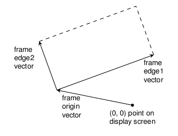
Tikz code here
We will use coordinates in the unit square ($0\le x,y\le 1$) to specify images. With each frame, we associate a frame coordinate map, which will be used to shift and scale images to fit the frame. The map transforms the unit square into the frame by mapping the vector $\boldsymbol v=(x,y)$ to the vector sum
For example, $(0,0)$ is mapped to the origin of the frame, $(1,1)$ to the vertex diagonally opposite , and $(0.5,0.5)$ to the centre of the frame. We can create a frame’s coordinate map with the following proceure:
(define (frame-coord-map frame)
  (lambda (v)
    (add-vert
      (origin-frame frame)
      (add-vect (scale-vect (xcor-vect v)
                            (edge1-frame frame))
                (scale-vect (ycor-vect v)
                            (edge2-frame frame))))))
Observe that applying frame-coord-map to a frame returns a procedure
that, given a vector, returns a vector. If the argument vector is in
the unit square, the result vector will be in the frame. For example,
((frame-coord-map a-frame) (make-vect 0 0))returns the same vector as
(origin-frame a-frame)Painters
A painter is represented as a procedure that, given a frame as
argument, draws a particular image shifted and scaled to fit the frame.
That is to say, if p is a painter and f is a frame, then we
produce p’s image in f by calling p with f as argument.
The details of how primitive painters are implemented depend on the
particular characteristics of the graphics system and the type of
image to be drawn. For instance, suppose we have a procedure
draw-line that draws a line on the screen between two specified
points. Then we can create painters fro line drawings, such as the
wave painter, from a list of line segments as follows:
(define (segments->painter segment-list)
  (lambda (frame)
    (for-each
      (lambda (seqment)
        (draw-line
         ((frame-coord-map frame) (start-segment segment))
         ((frame-coord-map frame) (end-seqment segment))))
      segment-list)))
The segments are given using coordinates with respect to the unit square. For each segment in the list, the painter transforms the segment endpoints with the frame coordinate map and draws a line between the transformed points.
Representing painters as procedures erects a powerful abstraction barrier in the picture language. We can create and intermix all sorts of primitive painters, based on a variety of graphics capabilities. The details of their implementation do not matter. Any procedure can serve as a painter, provided that it takes a frame as argument and draws something scaled to fit the frame.
Transforming and combining painters
An opeartion on painters (such as flip-vert or beside) works by
creating a painter that invokes the original painters with respect to
frames derived from the argument frame. Thus, for example, flip-vert
doesn’t have to know how a painter works in order to flip it – it
just has to know how to turn a frame upside down: the flipped painter
just uses the original painter, but in the inverted frame.
Painter operations are base on the procedure transform-painter,
which takes as arguments a painter and information on how to transform
a frame and produce a new painter. The transformed painter, when
called on a frame, transforms the frame and calls the original
painter on the transformed frame. The arguments to transform-painter
are points (represented as vectors) that specify the corners of the
new frame: when mapped into the new frame, the first point specifies
the new frame’s origin and the other two specify the ends of its edge
vectors. Thus, arguments within the unit square specify a frame
contained within the original frame.
(define (transform-painter painter origin corner1 corner2)
  (lambda (frame)
    (let ((m (frame-coord-map frame)))
      (let ((new-origin (m origin)))
        (painter
          (make-frame new-origin
                      (sub-vect (m corner1) new-origin)
                      (sub-vect (m corner2) new-origin)))))))
Here’s how to flip painter images vertically:
(define (flip-vert painter)
  (transform-painter painter
                     (make-vect 0.0 1.0)    ;new origin
                     (make-vect 1.0 1.0)    ;new end of edge1
                     (make-vect 0.0 0.0)))  ;new end of edge2
Using transform-painter, we can easily define new transformations.
For example, we can define a painter that shrinks its image to the
upper right quater of the frame it is given
(define (shrink-to-upper-right)
  (transform-painter painter
                     (make-vect 0.5 0.5)
                     (make-vect 1.0 0.5)
                     (make-vect 0.5 1.0)))
Other transformations rotate images counterclockwise by 90 degrees
(define (rotate90 painter)
  (transform-painter painter
                     (make-vect (1.0 0.0))
                     (make-vect (1.0 1.0))
                     (make-vect (0.0 0.0))))
or squash images towards the center of the frame:
(define (squash-inwards painter)x)
  (transform-painter painter
                     (make-vect 0.0 0.0)
                     (make-vect 0.65 0.35)
                     (make-vect 0.35 0.65)))
Frame transformation is also the key to defining means of combining
two or more painters. The beside procedure, for example, takes two
painters, transforms them to paint in the left and right halves of an
argument frame respectively, and procedures a new, compound painter.
When the compound painter is given a frame, it calls the first
transformed painter to paint in the left half of the frame and calls
the second transformed painter to paint in the right half of the frame:
(define (beside painter1 painter2)
  (let ((split-point (make-vect 0.5 0.0)))
    (let ((paint-left
           (transform-painter painter1
                              (make-vect 0.0 0.0)
                              split-point
                              (make-vect 0.0 1.0)))
          (paint-right
           (transform-painter painter2
                              split-point
                              (make-vect 1.0 0.0)
                              (make-vect 0.5 1.0))))
       (lambda (frame)
         (paint-left frame)
         (paint-right frame)))))
Levels of language for robust deisgn
In the picture langauge examples we have been introduced to the idea of stratified design, that is, the notion that a complex system should be structured as a sequence of levels that are described using a sequence of languages. Each level is construcuted by combining parts that are regarded as primitive at that level, and the parts that are constructed at each level are used as primitives at the next level. The langauge used at each level of a statified design has primitives, manes of combination, and means of abstraction appropriate to that level of detail.
Statified design helps make programs robust, that is, it makes it likely that small changes in a specification will require correspondingly small changes in the programs. In general, each level of a statified design provides a different vocabulary for expresing the characteristics of the system, and a different kind of ability to change it.